

Machine Learning: Heart Disease Prediction
Table of Contents
Introduction
Heart disease is a major health issue due to its high frequency and associated risks. Machine Learning can support diagnostics by identifying patterns in clinical data, improving early detection without replacing medical judgment.
This content will showcase a classification model in Python capable of predicting the probability of heart disease in a patient based on their clinical data.
Dataset Description
Dataset used: https://www.kaggle.com/datasets/johnsmith88/heart-disease-dataset/data
- Dataset size: 1025 (302 without duplicates)
- Features: 13
- Target feature: target (heart disease)
Feature descriptions:
age: Patient's age.
sex: Sex (1 = male, 0 = female).
cp: Chest pain type (4 values).
trestbps: Resting blood pressure.
chol: Serum cholesterol in mg/dl.
fbs: Fasting blood sugar > 120 mg/dl (1 = True, 0 = False).
restecg: Resting electrocardiographic results (0, 1, 2).
thalach: Maximum heart rate achieved.
exang: Exercise-induced angina (1 = Yes, 0 = No).
oldpeak: ST depression induced by exercise relative to rest.
slope: The slope of the peak exercise ST segment.
ca: Number of major vessels (0-3) colored by fluoroscopy.
thal: Thalassemia results (0 = normal; 1 = fixed defect; 2 = reversible defect).
target: Heart disease (0 = No, 1 = Yes).
Libraries
The libraries used for this project are the following:
# Loading dataset
import pandas as pd
import numpy as np
# Visualisation
import matplotlib.pyplot as plt
import seaborn as sns
# Preprocessing
from sklearn.preprocessing import OneHotEncoder
from sklearn.model_selection import train_test_split
from sklearn.compose import ColumnTransformer
# Report
from sklearn.metrics import accuracy_score, classification_report, confusion_matrix, roc_curve, auc
# Extra libraries
import sys, signal, copy, math
EDA (Exploratory Data Analysis)
Before training a model, it is important to analyze and visualize the dataset to understand its information, shape, behavior, and to detect potential issues. The goal of EDA is to ensure the data has the necessary quality for the model to learn correctly.
Initial Analysis
Let’s first process the CSV file to extract basic information.
# === Code === #
dataset = pd.read_csv('../dataset/heart.csv')
dataset.info()

# === Output === #
RangeIndex: 1025 entries, 0 to 1024
Data columns (total 14 columns):
 #   Column    Non-Null Count  Dtype
---  ------    --------------  -----
 0   age       1025 non-null   int64
 1   sex       1025 non-null   int64
 2   cp        1025 non-null   int64
 3   trestbps  1025 non-null   int64
 4   chol      1025 non-null   int64
 5   fbs       1025 non-null   int64
 6   restecg   1025 non-null   int64
 7   thalach   1025 non-null   int64
 8   exang     1025 non-null   int64
 9   oldpeak   1025 non-null   float64
 10  slope     1025 non-null   int64
 11  ca        1025 non-null   int64
 12  thal      1025 non-null   int64
 13  target    1025 non-null   int64
dtypes: float64(1), int64(13)
Anotations:
- There are 1025 samples and 14 columns in total (one representing the final diagnosis indicating the presence or absence of heart issues).
- There are no missing values (non-null). This is good as it saves preprocessing effort.
- All features are numeric (int64 and float64).
Descriptive Statistics:
# === Code === #
dataset.describe()

# === Output === #
               age          sex           cp     trestbps  ...        slope           ca         thal       target
count  1025.000000  1025.000000  1025.000000  1025.000000  ...  1025.000000  1025.000000  1025.000000  1025.000000
mean     54.434146     0.695610     0.942439   131.611707  ...     1.385366     0.754146     2.323902     0.513171
std       9.072290     0.460373     1.029641    17.516718  ...     0.617755     1.030798     0.620660     0.500070
min      29.000000     0.000000     0.000000    94.000000  ...     0.000000     0.000000     0.000000     0.000000
25%      48.000000     0.000000     0.000000   120.000000  ...     1.000000     0.000000     2.000000     0.000000
50%      56.000000     1.000000     1.000000   130.000000  ...     1.000000     0.000000     2.000000     1.000000
75%      61.000000     1.000000     2.000000   140.000000  ...     2.000000     1.000000     3.000000     1.000000
max      77.000000     1.000000     3.000000   200.000000  ...     2.000000     4.000000     3.000000     1.000000
By analyzing the dataset statistics, the following conclusions can be drawn:
- Diagnosis integrity: The target column (final diagnosis) only contains 0s and 1s, with no invalid values.
- Balanced dataset: The target column shows a mean of 0.51, meaning 51.3% of the patients have heart disease and 48.7% do not. Balancing techniques will not be necessary.
- Gender imbalance: 69.5% of the samples are male and 30.5% are female. The model will have more experience evaluating male patients.
- Age distribution: A large portion of the patients (between the 25th and 75th percentiles) are clustered between 48 and 61 years old.
- Scale differences: Values in columns like trestbps reach up to 200, while others like cp range from 0 to 3. This will require data scaling later on.
- Categorical data: There are numerical columns representing nominal categories (such as chest pain type). If left as is, the model might incorrectly assume a “type 3” pain is mathematically worth more than a “type 1” pain.
Before continuing with the analysis, basic cleaning will be performed, and columns will be renamed to be more descriptive.
# Drop duplicates
dataset = dataset.drop_duplicates()

# Rename columns
dataset = dataset.rename(columns={
	'age': 'Age',
	'sex': 'Sex',
	'cp': 'Chest Pain Type',
	'trestbps': 'Resting BP',
	'chol': 'Cholesterol',
	'fbs': 'Fasting Blood Sugar',
	'restecg': 'Resting ECG',
	'thalach': 'Max Heart Rate',
	'exang': 'Exercise Induced Angina',
	'oldpeak': 'ST Depression',
	'slope': 'ST Slope',
	'ca': 'Num Major Vessels',
	'thal': 'Thalassemia Results',
	'target': 'Heart Disease'
})
After removing duplicated rows, the dataset went from 1025 to 302 samples.
Visual Analysis
Column histograms:
# === Code === #
dataset.hist(figsize=(15, 10), bins=20)
plt.tight_layout()
plt.show()
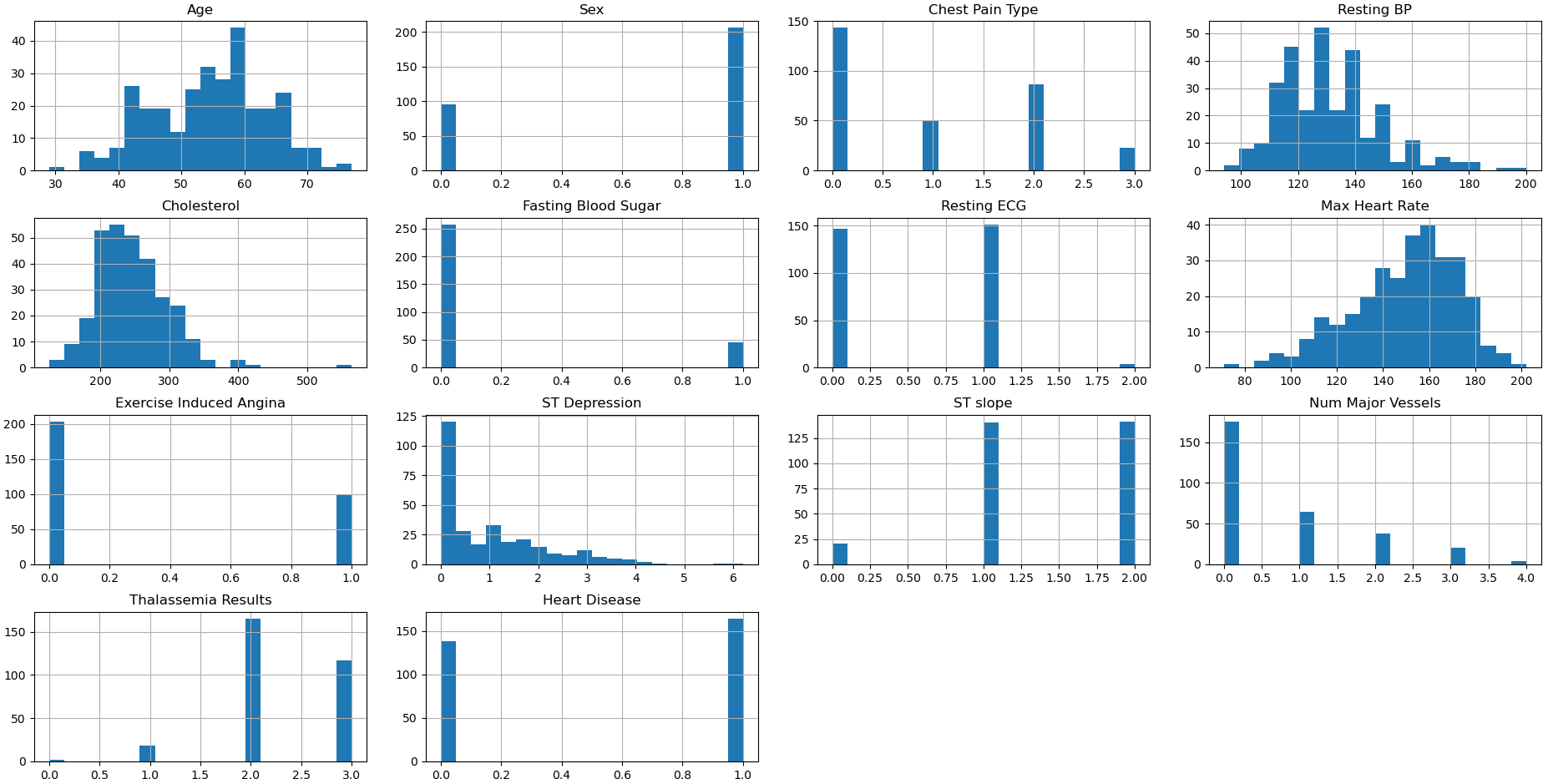
A histogram is useful for getting an overview of the data. It leads to the following conclusions:
- The presence of numerical categories is confirmed (e.g., Sex, Exercise Ind. Ang., Chest Pain).
- Possible outliers are observed in the ST Depression and Cholesterol columns. Although both show a normal (bell-shaped) curvature, there are isolated data points far from the normal distribution.
Cholesterol Boxplot:
# === Code === #
sns.boxplot(x="Heart Disease", y="Cholesterol", data=dataset)
plt.title("Heart Disease vs Cholesterol")
plt.show()
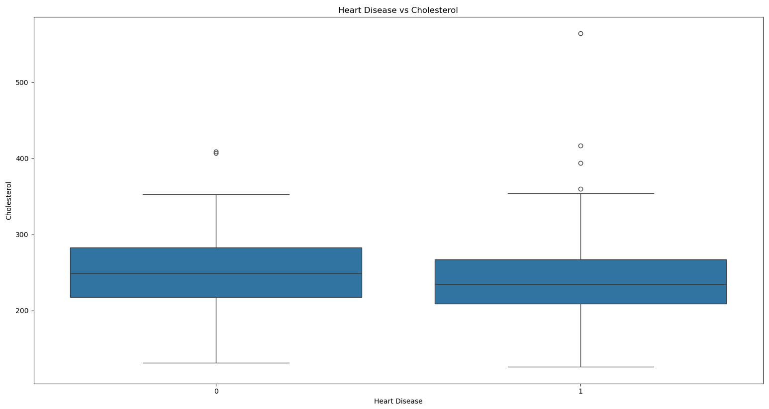
To confirm the outliers in the Cholesterol feature, a boxplot is used. Conclusions:
- A very high cholesterol value exceeding 500 mg/dl is noted. Since it is a rare (but clinically possible) value, it will be handled later to prevent excessive noise.
- The medians between healthy and sick patients are similar. This means cholesterol does not have a strong correlation with the final prediction on its own.
ST Depression Boxplot:
# === Code === #
sns.boxplot(x="Heart Disease", y="ST Depression", data=dataset)
plt.title("Heart Disease vs ST depression")
plt.show()
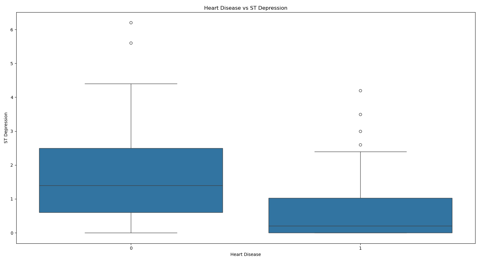
Conclusions:
- Both types of patients present outliers, but they are not problematic because they are not erroneous values and are clinically possible.
- At first glance, it can be noted that the data distribution for healthy patients is more dispersed and the median is higher than the median for sick patients.
Column Heatmap:
# === Code === #
plt.figure(figsize=(12,8))
sns.heatmap(dataset.corr(), annot=True, cmap="Blues")
plt.show()
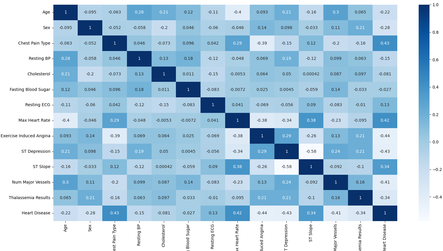
This chart is highly useful as it reveals which variables carry the most weight for the final prediction. Analysis yields the following conclusions:
- Positive correlations: Several features show a high correlation with the final prediction; the higher their value, the higher the probability of disease. Notable among them are Chest Pain Type (0.43), Max Heart Rate (0.42), and ST Slope (0.34).
- Negative correlations: There are also features with strong negative correlation; as their value increases, the likelihood of the patient being healthy increases. Highlights include Exercise Ind. Ang. (-0.44), ST Depression (-0.43), Num Maj. Ves. (-0.41), and Thalassemia Results (-0.34).
- Multicollinearity: Although there are strong correlations between some features, such as ST Slope and ST Depression (-0.58), they remain within a safe range for the model and do not present a severe multicollinearity issue.
Preprocessing
After a preliminary diagnosis of the data, preprocessing is used to perform the necessary modifications and transformations for the model.
Before processing and training, it is crucial to split the dataset into training and test sets to prevent Data Leakage.
# Optional: Rename numerical values to nominal ones
mapping = {
    'Sex': {
        0: 'Female',
        1: 'Male'
    },
    'Chest Pain Type': {
        0: 'Typical angina',
        1: 'Atypical angina',
        2: 'Non-anginal pain',
        3: 'Asymptomatic'
    },
    'Fasting Blood Sugar': {
        0: '< 120 mg/dl',
        1: '> 120 mg/dl'
    },
    'Resting ECG': {
        0: 'Normal',
        1: 'ST-T wave abnormality',
        2: 'Left ventricular hypertrophy'
    },
    'Exercise Induced Angina': {
        0: 'No',
        1: 'Yes'
    },
    'ST Slope': {
        0: 'Upsloping',
        1: 'Flat',
        2: 'Downsloping'
    },
    'Thalassemia Results': {
        0: 'Normal',
        1: 'Fixed Defect',
        2: 'Reversible Defect',
        3: 'Unknown'
    }
}
for column, values in mapping.items():
    dataset[column] = dataset[column].replace(values)
print("+ Variables renamed.")

# Separate features (X) and target (y)
X = dataset.drop(columns=['Heart Disease'])
y = dataset['Heart Disease']

# Split dataset into training and test data
X_train, X_test, y_train, y_test = train_test_split(
	X, y,
	test_size=0.2, # 20% of the data will be used for testing
	shuffle=True,
	random_state=123,
	stratify=y
)
The first issue to tackle is nominal categories. Converting textual values prevents training errors, and transforming discrete numeric identifiers (e.g., 0 = female, 1 = male) prevents the model from assigning heavier mathematical weight to larger numbers.
The chosen method is One-Hot Encoding, which converts categorical data into binary. For example, in the Sex column containing Male and Female, two independent columns will be created (sex_male and sex_female), each with a binary value identifying the trait.
categorical_cols = ['Sex', 'Chest Pain Type', 'Fasting Blood Sugar', 'Resting ECG', 'Exercise Induced Angina', 'ST Slope', 'Num Major Vessels', 'Thalassemia Results']
preprocessor = ColumnTransformer(transformers=[('onehot', OneHotEncoder(handle_unknown='ignore', sparse_output=False), categorical_cols)], remainder='passthrough', verbose_feature_names_out=False)

# One-Hot encoding on training data
encoded_data = preprocessor.fit_transform(X_train)
X_train = pd.DataFrame(encoded_data, columns=preprocessor.get_feature_names_out(), index=X_train.index)

# One-Hot Encoding on test data
encoded_test = preprocessor.transform(X_test)
X_test = pd.DataFrame(encoded_test, columns=preprocessor.get_feature_names_out(), index=X_test.index)
To handle outliers, the Capping (or Winsorizing) method at the 99th percentile will be used on Cholesterol. This method calculates the maximum value where 99% of the data sits and limits those atypical values that exceed this boundary. For instance, if 99% of the data falls under 410, outliers (like 520) will be capped at the defined limit.
# Winsorizing training data
upper_limit = X_train['Cholesterol'].quantile(0.99)
X_train['Cholesterol'] = np.where(
    X_train['Cholesterol'] > upper_limit,
    upper_limit,
    X_train['Cholesterol']
)

# Winsorizing test data
X_test['Cholesterol'] = np.where(
    X_test['Cholesterol'] > upper_limit, # Same limit to avoid Data Leakage
    upper_limit,
    X_test['Cholesterol']
)
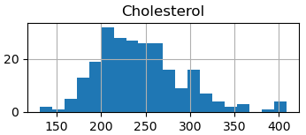
After applying Capping, the extreme outlier was capped to a value close to 400.
Finally, to resolve the discrepancy in numerical ranges among features, Z-Score Normalization scaling will be implemented. This ensures all continuous variables share a standardized scale, preventing the model from giving undue importance to features simply because they have larger numbers.
def zscore_normalize(X, mu=None, sigma=None):
    X_norm = X.copy()
    scaling_features = ['Age', 'Resting BP', 'Cholesterol', 'Max Heart Rate', 'ST Depression']
    if mu is None or sigma is None:
        mu = X[scaling_features].mean()
        sigma = X[scaling_features].std()

    X_norm[scaling_features] = (X[scaling_features] - mu) / sigma

    return mu, sigma, X_norm

mu, sigma, X_train = zscore_normalize(X_train)
Model Training
To solve this classification problem, Logistic Regression trained with Gradient Descent will be used.
Logistic Regression is an algorithm used to make binary class predictions (Yes or No). Its operation relies on two main steps:
- Linear Regression: Calculates the weighted sum of the input features. The formula is: $z = \vec{w} \cdot \vec{x}$ or $z = w_1x_1 + w_2x_2 + \dots + w_nx_n + b$, where $x_j$ represents each feature and $w_j$ is its weight or importance.
- Sigmoid Function: Takes the result of the previous step and passes it through the Sigmoid Function (or Logistic Function), which converts any number to a value between 0 and 1. The formula is $g(z) = \frac{1}{1+e^{-z}}$.
Python implementation:
def logistic_regression(X, w, b):
    m = X.shape[0]

    y_hat = []
    for i in range(m):
        z = np.dot(w, X[i]) + b
        g = 1 / (1 + np.exp(-z))
        y_hat.append(g)

    return y_hat
The arguments w and b correspond to the model’s weights and define how well it will perform and make predictions.
The Cost Function measures how wrong or distant the model's predictions are compared to the actual diagnoses.
The distance between each prediction and the diagnosis is called loss, and the sum of all of them is called cost. During training, gradient descent will adjust the parameters (w and b) to minimize this loss and improve the model’s quality.
The function used to calculate the loss is the following:
- $L(f_{\vec{w},b}(\vec{x}^{(i)}), y^{(i)}) = -y^{(i)} \log(f_{\vec{w},b}(\vec{x}^{(i)})) - (1 - y^{(i)}) \log(1 - f_{\vec{w},b}(\vec{x}^{(i)}))$
Where:
- $f_{\vec{w},b}(\vec{x}^{(i)}) = g(z) = \frac{1}{1+e^{-z}}$
This helps build the simplified Cost Function:
- $J(\vec{w},b) = \frac{1}{m} \sum_{i=1}^m [L(f_{\vec{w},b}(\vec{x}^{(i)}), y^{(i)})]$
Python implementation:
def cost_function(X, y, w, b):
    m = X.shape[0]

    loss = 0.
    for i in range(m):
        z = np.dot(w, X[i]) + b
        f_wb = 1 / (1 + np.exp(-z))
        loss += -y[i] * np.log(f_wb) - (1 - y[i]) * np.log(1 - f_wb)

    loss /= m
    return loss
Gradient Descent is used to minimize a function. In this model, it will be ideal for minimizing the Cost Function to obtain suitable parameters (`w` and `b`).
The algorithm is as follows:
$\text {repeat until convergence: } \lbrace \\ \; w := w-\alpha \frac\delta {\delta w}J(w,b) \\ \; b := b-\alpha \frac \delta{\delta b}J(w,b) \\ \rbrace$
According to calculus rules, this equals:
$w := w-\alpha \frac1m \sum_{i=1}^m (f_{w,b}(x^{(i)}) - y^{(i)}) x^{(i)}$
$b := b-\alpha \frac1m \sum_{i=1}^m (f_{w,b}(x^{(i)}) - y^{(i)})$
These algorithms update the parameters (w, b) by subtracting a learning rate ($\alpha$) multiplied by the partial derivative ($\frac{\partial}{\partial w}J(w,b)$). Each update represents a small step taken downwards until convergence is reached (no more significant changes in w and b).
Python implementation:
def compute_gradient(X, y, w, b):
    m, n = X.shape
    dj_w = np.zeros((n,))
    dj_b = 0.

    for i in range(m):
        z = np.dot(w, X[i]) + b
        f_wb = 1 / (1 + np.exp(-z))
        error = f_wb - y[i]

        for j in range(n):
            dj_w[j] += error * X[i, j]

        dj_b += error

    dj_w /= m
    dj_b /= m

    return dj_w, dj_b

def gradient_descent(X, y, w_ini, b_ini, iterations, alpha):
    w = copy.deepcopy(w_ini)
    b = 0.
    J_history = []

    for i in range(iterations):
        dj_w, dj_b = compute_gradient(X, y, w, b)

        w = w - alpha * dj_w
        b = b - alpha * dj_b

        # Show progress
        if i < 100000:
            J_history.append(cost_function(X, y, w, b))
        if i % math.ceil(iterations / 10) == 0:
            print(f" Iteration {i:4d}: Cost {J_history[-1]}")

    return w, b
The learning rate ($\alpha$) is a positive value used to control how large the step will be in each iteration. If the value is too small, the algorithm will be slow, but if it's too large, it could overshoot the minimum, increase the cost, and never find the global minimum.
To find the appropriate value, the following steps can be followed:
- Start with a very low value, like 0.001, and check the cost graph (learning curve).
- If it is too slow, increase its size threefold (e.g., 0.003, 0.01, 0.03, 0.1, 0.3, 1, etc.) manually until finding a value so high that it causes the cost to increase.
- After establishing very low and very high thresholds, slowly narrow down to the highest value that consistently decreases the cost.
Analysis for $\alpha = 0.001$:
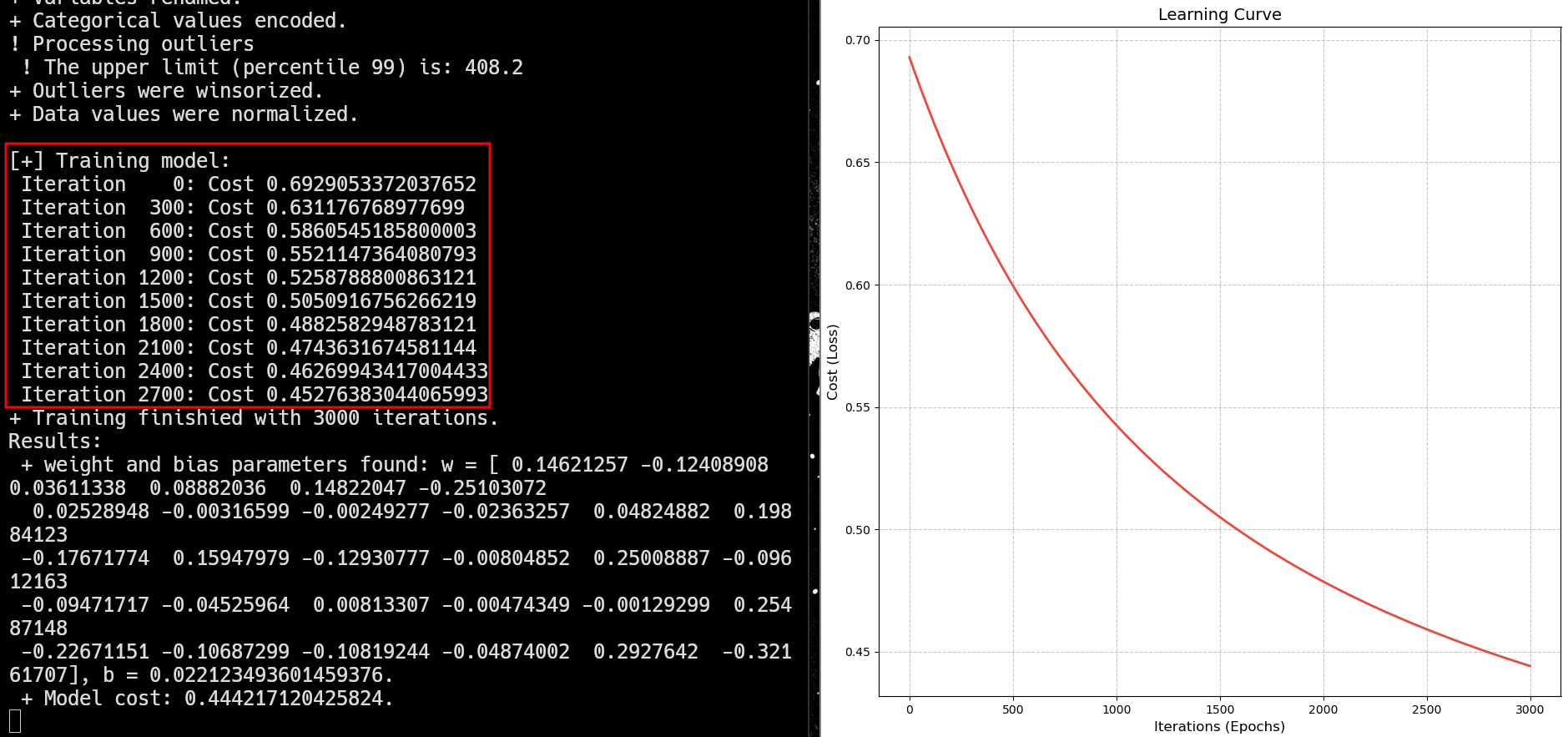
- The cost decreases little by little in each iteration; however, it is a very slow process.
- From iteration 2100 to 2700, there have been noticeable cost decreases, meaning it hasn’t reached convergence yet.
Analysis for $\alpha = 0.003$:
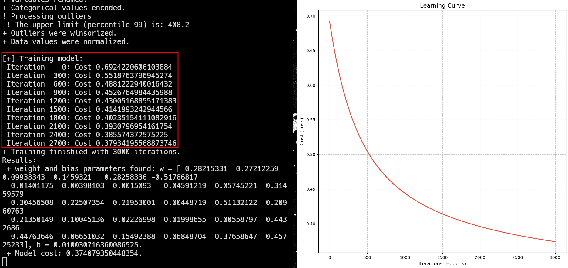
- By increasing the learning rate size threefold (0.003), it is noticeable that the learning curve took a steeper shape.
- The slope indicates a large cost decrease in fewer iterations. Even so, it remains slow because notable cost drops still occur in the final iterations.
Analysis for $\alpha = 1.0$:
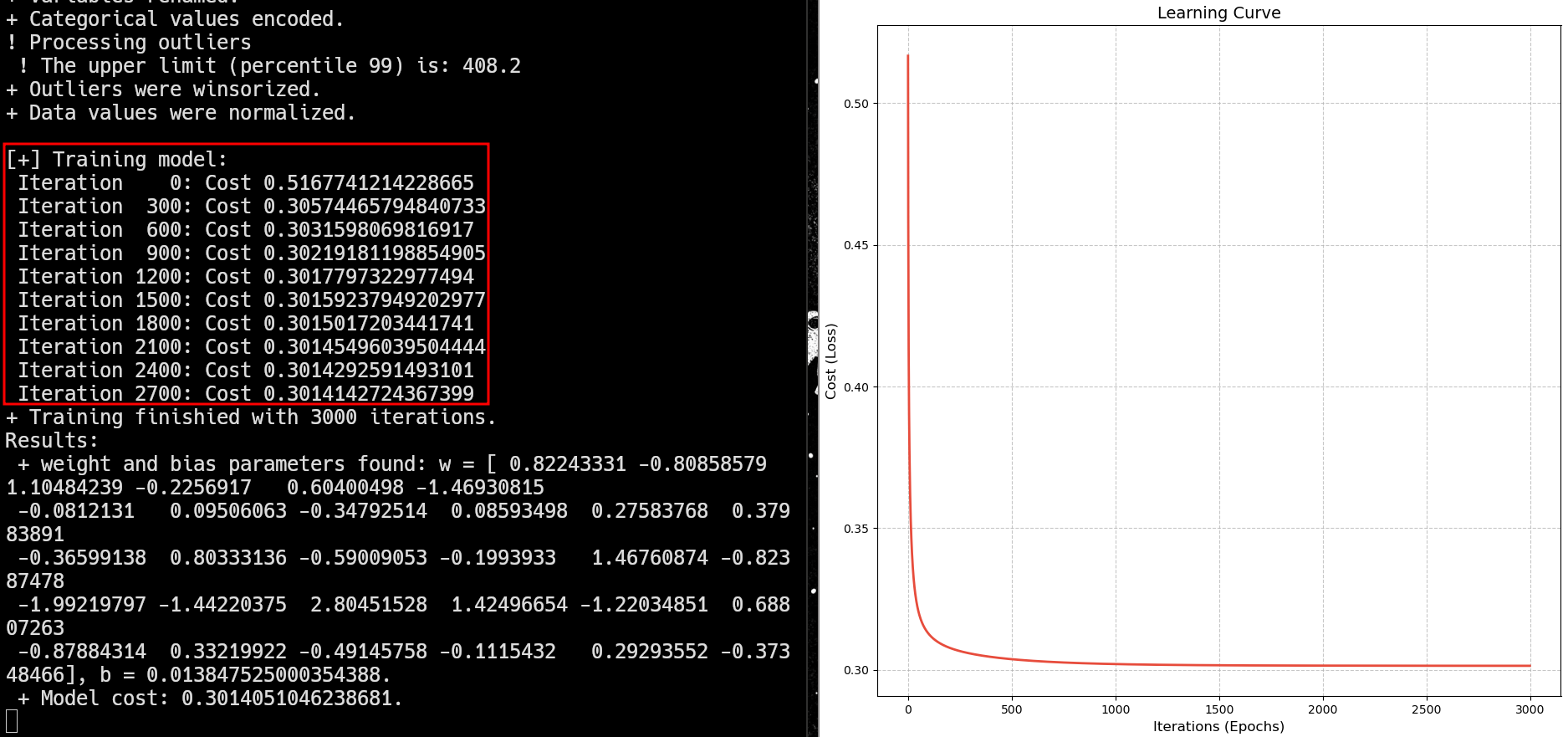
- The final selected $\alpha$ value for this model is 1.0, and as seen in the graph, it forms an even steeper line.
- The learning curve decreases rapidly in the first 300 iterations and uniformly flattens out.
- Between 2100 and 2700 iterations, the cost stops decreasing considerably, indicating convergence has been reached, making it an optimal value for the model.
Putting all the pieces together results in the complete training script.
#!/usr/bin/env python

# Load dataset
import pandas as pd
import numpy as np
# Visualisation
import matplotlib.pyplot as plt
import seaborn as sns
# Preprocessing
from sklearn.preprocessing import OneHotEncoder
from sklearn.model_selection import train_test_split
from sklearn.compose import ColumnTransformer
# Report
from sklearn.metrics import accuracy_score, classification_report, confusion_matrix, roc_curve, auc
# Extra libraries
import sys, signal, copy, math

# ====
# HELPER FUNCTIONS
# ====
def ctrlc_handler(sig, frame):
    print("\n[!] Exiting.")
    sys.exit(0)
signal.signal(signal.SIGINT, ctrlc_handler)

dataset = pd.read_csv('../datasets/heart.csv')

def zscore_normalize(X, mu=None, sigma=None):
    X_norm = X.copy()
    scaling_features = ['Age', 'Resting BP', 'Cholesterol', 'Max Heart Rate', 'ST Depression']
    if mu is None or sigma is None:
        mu = X[scaling_features].mean()
        sigma = X[scaling_features].std()

    X_norm[scaling_features] = (X[scaling_features] - mu) / sigma

    return mu, sigma, X_norm

def logistic_regression(X, w, b):
    m = X.shape[0]

    y_hat = []
    for i in range(m):
        z = np.dot(w, X[i]) + b
        g = 1 / (1 + np.exp(-z))
        y_hat.append(g)

    return y_hat

def cost_function(X, y, w, b):
    m = X.shape[0]

    loss = 0.
    for i in range(m):
        z = np.dot(w, X[i]) + b
        f_wb = 1 / (1 + np.exp(-z))
        loss += -y[i] * np.log(f_wb) - (1 - y[i]) * np.log(1 - f_wb)

    loss /= m
    return loss

def compute_gradient(X, y, w, b):
    m, n = X.shape
    dj_w = np.zeros((n,))
    dj_b = 0.

    for i in range(m):
        z = np.dot(w, X[i]) + b
        f_wb = 1 / (1 + np.exp(-z))
        error = f_wb - y[i]

        for j in range(n):
            dj_w[j] += error * X[i, j]

        dj_b += error

    dj_w /= m
    dj_b /= m

    return dj_w, dj_b

def gradient_descent(X, y, w_ini, b_ini, iterations, alpha):
    w = copy.deepcopy(w_ini)
    b = 0.
    J_history = []

    for i in range(iterations):
        dj_w, dj_b = compute_gradient(X, y, w, b)

        w = w - alpha * dj_w
        b = b - alpha * dj_b

        # Show progress
        if i < 100000:
            J_history.append(cost_function(X, y, w, b))
        if i % math.ceil(iterations / 10) == 0:
            print(f" Iteration {i:4d}: Cost {J_history[-1]}")

    return w, b, J_history

# ====
# PREPROCESSING
# ====
print("[+] Preprocessing:")
print(f"+ Cleaned up {dataset.duplicated().sum()} duplicated values.")
dataset = dataset.drop_duplicates()

dataset = dataset.rename(columns={
    'age': 'Age',
    'sex': 'Sex',
    'cp': 'Chest Pain Type',
    'trestbps': 'Resting BP',
    'chol': 'Cholesterol',
    'fbs': 'Fasting Blood Sugar',
    'restecg': 'Resting ECG',
    'thalach': 'Max Heart Rate',
    'exang': 'Exercise Induced Angina',
    'oldpeak': 'ST Depression',
    'slope': 'ST Slope',
    'ca': 'Num Major Vessels',
    'thal': 'Thalassemia Results',
    'target': 'Heart Disease'
})
mapping = {
    'Sex': {
        0: 'Female',
        1: 'Male'
    },
    'Chest Pain Type': {
        0: 'Typical angina',
        1: 'Atypical angina',
        2: 'Non-anginal pain',
        3: 'Asymptomatic'
    },
    'Fasting Blood Sugar': {
        0: '< 120 mg/dl',
        1: '> 120 mg/dl'
    },
    'Resting ECG': {
        0: 'Normal',
        1: 'ST-T wave abnormality',
        2: 'Left ventricular hypertrophy'
    },
    'Exercise Induced Angina': {
        0: 'No',
        1: 'Yes'
    },
    'ST Slope': {
        0: 'Upsloping',
        1: 'Flat',
        2: 'Downsloping'
    },
    'Thalassemia Results': {
        0: 'Normal',
        1: 'Fixed Defect',
        2: 'Reversible Defect',
        3: 'Unknown'
    }
}
for column, values in mapping.items():
    dataset[column] = dataset[column].replace(values)
print("+ Variables renamed.")

# Split dataset
X = dataset.drop(columns=['Heart Disease'])
y = dataset['Heart Disease']
X_train, X_test, y_train, y_test = train_test_split(X, y, test_size=0.2, shuffle=True, random_state=123, stratify=y)

# Encode categorical values (One-Hot Encoding)
categorical_cols = ['Sex', 'Chest Pain Type', 'Fasting Blood Sugar', 'Resting ECG', 'Exercise Induced Angina', 'ST Slope', 'Num Major Vessels', 'Thalassemia Results']
preprocessor = ColumnTransformer(transformers=[('onehot', OneHotEncoder(handle_unknown='ignore', sparse_output=False), categorical_cols)], remainder='passthrough', verbose_feature_names_out=False)
encoded_data = preprocessor.fit_transform(X_train)
X_train = pd.DataFrame(encoded_data, columns=preprocessor.get_feature_names_out(), index=X_train.index)

encoded_test = preprocessor.transform(X_test)
X_test = pd.DataFrame(encoded_test, columns=preprocessor.get_feature_names_out(), index=X_test.index)
print("+ Categorical values encoded.")

# Handle outliers (Winsorizing)
print("! Processing outliers")
upper_limit = X_train['Cholesterol'].quantile(0.99)
print(f" ! The upper limit (percentile 99) is: {upper_limit}")
X_train['Cholesterol'] = np.where(
    X_train['Cholesterol'] > upper_limit,
    upper_limit,
    X_train['Cholesterol']
)
X_test['Cholesterol'] = np.where(
    X_test['Cholesterol'] > upper_limit,
    upper_limit,
    X_test['Cholesterol']
)
print("+ Outliers were winsorized.")

# Z-score normalization
mu, sigma, X_train = zscore_normalize(X_train)
print("+ Data values were normalized.")

# ====
# TRAINING
# ====
# Configuration
X_train = X_train.to_numpy()
y_train = y_train.to_numpy()
iterations = 3000
alpha = 1.0
w = np.zeros((X_train.shape[1],))
b = 0.

# Gradient Descent
print("\n[+] Training model:")
w, b, J_history = gradient_descent(X_train, y_train, w, b, iterations, alpha)
cost = cost_function(X_train, y_train, w, b)
print(f"+ Training finishied with {iterations} iterations.")
print("Results:")
print(f" + weight and bias parameters found: w = {w}, b = {b}.")
print(f" + Model cost: {cost}.")

# Graphic learning curve
plt.figure(figsize=(10, 6))
plt.plot(range(len(J_history)), J_history, color='#e74c3c', linewidth=2)
plt.title('Learning Curve', fontsize=14)
plt.xlabel('Iterations (Epochs)', fontsize=12)
plt.ylabel('Cost (Loss)', fontsize=12)
plt.grid(True, linestyle='--', alpha=0.7)
plt.tight_layout()
plt.show()

# ===
# TESTING
# ===
print("\n[+] Testing:")
_, _, X_test = zscore_normalize(X_test, mu, sigma)
X_test = X_test.to_numpy()
y_test = y_test.to_numpy()

threshold = 0.5
y_probs = np.array(logistic_regression(X_test, w, b)) # Probabilities
y_hat = (y_probs >= threshold).astype(int)
Model Evaluation
To evaluate the model’s performance and precision, several methods and analyses will be conducted.
Confusion Matrix.
# === Code === #
sns.heatmap(confusion_matrix(y_test, y_hat), annot=True, fmt='d', cmap='Reds', annot_kws={'size': 24})
plt.show()
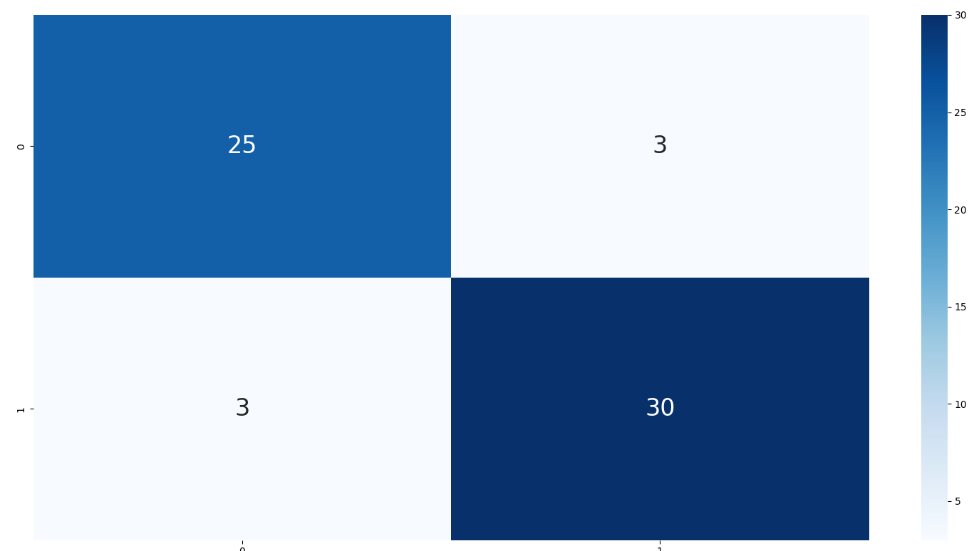
This chart compares the prediction outcomes against the actual diagnosis to see how wrong the model was. Results:
- The model produced 25 True Positives (TP) and 30 True Negatives (TN).
- Although the model correctly predicted the majority of the data, there were 3 False Negatives (FN). This is critical because, in this scenario, these are three patients (actually sick) that the model classified as healthy.
- Depending on the problem being solved and its criticality, it is often better to have more False Positives (FP) than False Negatives (FN). Here, it is better to falsely suspect disease in a healthy patient than to dismiss a sick patient as healthy.
- One attempt to mitigate this is by adjusting the decision threshold to prioritize detecting sick patients over healthy ones.
Classification Report.
# === Code === #
class_rep = classification_report(y_test, y_hat)
print(class_rep)

# === Output === #
              precision    recall  f1-score   support

           0       0.89      0.89      0.89        28
           1       0.91      0.91      0.91        33

    accuracy                           0.90        61
   macro avg       0.90      0.90      0.90        61
weighted avg       0.90      0.90      0.90        61
This report shows the model’s statistics to measure its general reliability and accuracy. Results:
- Precision: When the model declares a patient is sick, it is correct 91% of the time.
- Recall: Out of all the truly sick patients, it successfully detected 91%.
- F1-Score: The harmonic mean between the model’s precision and recall.
- Accuracy: The overall percentage of correct model predictions is 90%.
ROC Curve and AUC.
# === Code === #
fpr, tpr, umbrales = roc_curve(y_test, y_probs)
roc_auc = auc(fpr, tpr)

plt.figure(figsize=(8, 6))
plt.plot(fpr, tpr, color='#e74c3c', lw=2, label=f'ROC Curve (AUC = {roc_auc:.2f})')
plt.plot([0, 1], [0, 1], color='navy', lw=2, linestyle='--', label='Bad model (AUC = 0.50)')
plt.xlim([0.0, 1.0])
plt.ylim([0.0, 1.05])
plt.xlabel('FPR (False Positive Rate)')
plt.ylabel('Recall (True Positive Rate)')
plt.title('ROC (Receiver Operating Characteristic)')
plt.legend(loc="lower right")
plt.grid(True, linestyle='--', alpha=0.7)
plt.tight_layout()
plt.show()
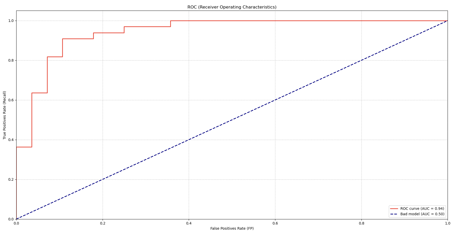
The ROC curve and the AUC area are tools used to demonstrate model quality. A good model should climb rapidly on the Y-axis.
- The obtained AUC (Area Under the Curve) is 0.94 (94%). This indicates an excellent probability that the model will correctly classify a patient’s heart disease.
Feature importance.
# === Code === #
importance = pd.DataFrame({
    'Feature': feature_names,
    'Weight': w
})
importance = importance.sort_values(by='Weight', key=abs, ascending=False)
plt.figure(figsize=(12, 8))
sns.barplot(x='Weight', y='Feature', data=importance, palette='vlag')
plt.title('Variable Importance (Linear Regression Weights)')
plt.xlabel('Weight')
plt.ylabel('Feature')
plt.grid(True, axis='x', linestyle='--', alpha=0.7)
plt.tight_layout()
plt.show()
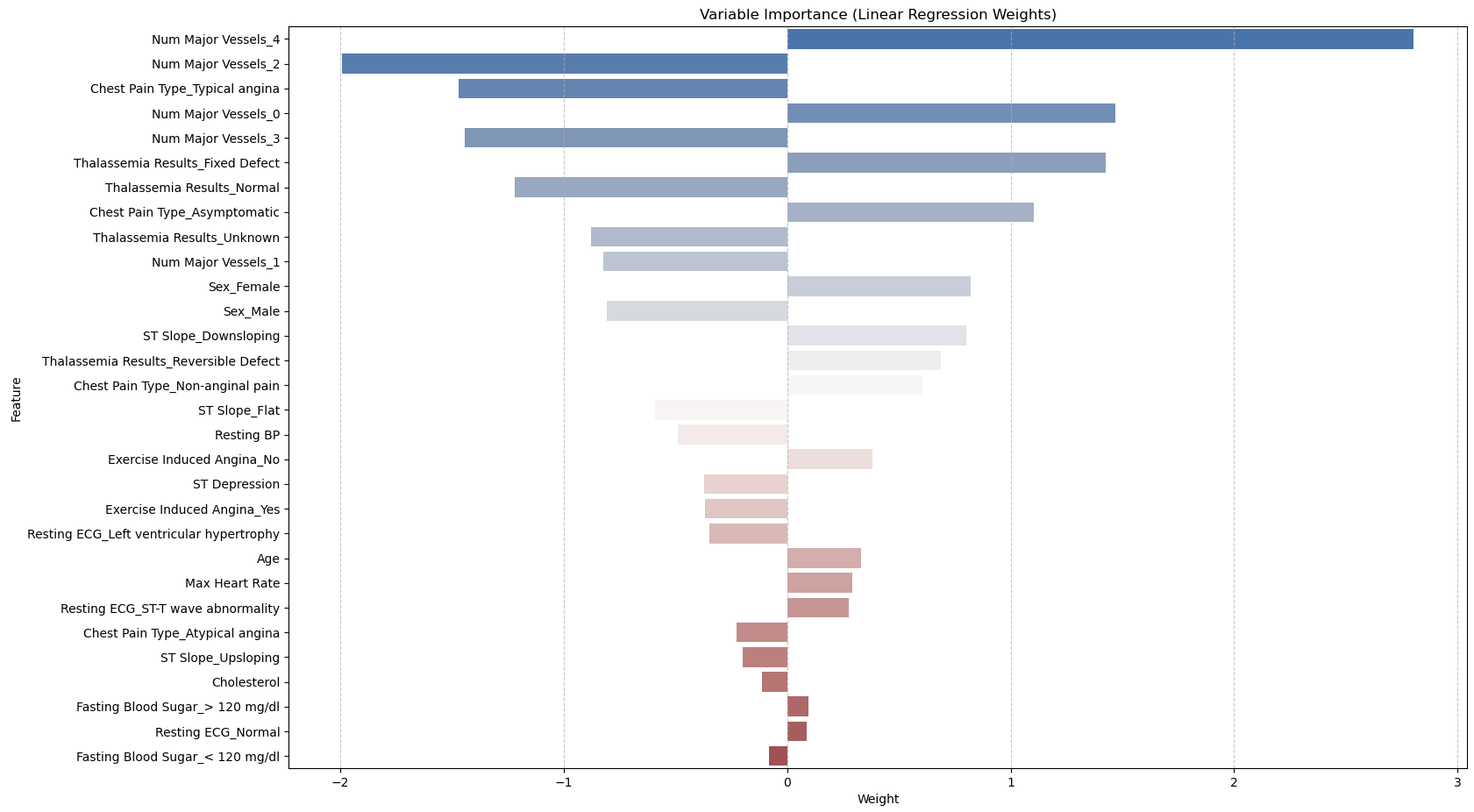
This chart shows the weights that hold more or less importance in the final prediction:
- Positive weights (bars to the right): Patients with high values in this feature increase their probability of being sick.
- Negative weights (bars to the left): Patients with high values in this feature increase their probability of being healthy.
- Weights near zero: This means the feature’s weight is practically irrelevant to the final prediction.